This week, let's talk about word clouds. You've probably seen them before - they're almost exactly what they sound like: single words arranged in a cloud-like formation, with the size of the words indicating how frequently they appear in the source material.
Word clouds are not exactly the most sophisticated analytical tools, but they are easily the most accessible way to analyze text in one go. Don't have the skill set to conduct k-means clustering on the term frequency-inverse document frequency matrix of a set of documents? Yeah, most people don't. But that shouldn't mean you can't get something out of a bunch of text.
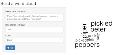
Power to the people! Programming background or no, you can use my free web app to create your own word cloud. Paste in or type any block of text, play with the other settings as you wish, and click run. If you'd like to save your word cloud, just right-click and save the image.
The app is hosted on the free version of shinyapps.io, meaning only 25 people will get to play with this app this month before I hit the instance limit - so don't delay! :)
Note: the code behind this app does some text-cleaning, meaning it strips out extra white space, punctuation, converts to lower case, and removes very common words like "the" and "and". So if you are typing in text and wondering why not everything is showing up, that may be why.
With this app you could, say, visualize text from the first presidential debate of 2016 ...
Combined word cloud from entire debate
Lester Holt's word cloud
Hillary Clinton's word cloud
Donald Trump's word cloud
Have fun!


